When you zoom out, free goods and services may cost us way more than expected.

How to create a false stereotype through sample bias.

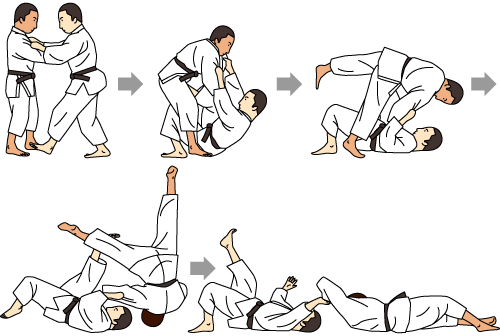
Sutemi-waza are a class of throws in jujitsu or aikido known as sacrifice throws. They are tricky, but very powerful: they work because of the opponent’s momentum.

There’s a game potential clients and advisors play, and I think everyone loses.

There’s a seduction in behavioral science: 'here’s a bias, go be better by not being biased'.